Above is a 2 sector model of the circular flow. In the model are households and firms with the firms producing goods and services by hiring labour and other factor inputs from households. Households supply their labour and buy consumer goods. In return for supplying factor inputs, households receive income (wages, rent, interest and dividend payments) which they spend on consumer goods.

This is a closed system and so the flows must balance. This shows the 3 methods of how GDP can be measured, by incomes, by total amount of output, or by total expenditure.

In reality there are leakages (or withdrawals) from the circular flow so in practise it isn’t a closed system. These leakages are savings, tax and imports. If money is saved then it doesn’t contribute to AD. If the government takes money away from the economy or doesn’t spend it, or similarly if there are more imports than exports then the economy will slow down. These 3 leakages determine the size of the multiplier.

There are also 3 injections into the circular flow. These are investment, government spending and exports.

(T)=Tax, (S) = Savings, (M) = Imports, (G) = Government Spending, (I) = Investment, (X) = Exports

Aggregate Demand

Aggregate demand (AD) is the demand side of the economy, and if all the agents demanding goods and services in an economy are added together (aggregate means total) then we have GDP. AD varies between seasons, for example there is more consumer demand for goods at Christmas than in early January. Ergo there are seasonal fluctuations in GDP, generally these differences are removed from headline figures to prevent confusion.

Aggregate demand can be given by the equation Y = C + I + G + (X-M) where Y is national income (GDP), C is consumption, I is investment in capital, G is government spending and (X-M) is exports minus imports; also known as net exports. These individual items which account for GDP are known as components. This equation is called the national income accounts identity.

The price level is measured by the GDP deflator index. It is similar to CPI and RPI but includes industrial prices. You can read more about the GDP deflator on the Inflation page.

As we can see the aggregate demand curve is downward sloping, there are 3 reasons for this.

The first is International Competitiveness. If the prices in one economy are high or they rise then its goods and services are less competitive against its foreign rivals and this will lower demand for exports contributing to a decrease in GDP ceteris paribus. This means if inflation is high then real output will be low. Conversely if inflation is low then real output will be higher.

The real balance effect is where a rise in the price level will reduce the real value of income and wealth and vice versa with a fall in the price level. If there is a fall in the value of real income and wealth (when inflation is high) then consumption will fall as the spending power of income will be reduced causing less output.

The third reason is the interest rate effect. The BoE MPC reduces inflation by raising the rate of interest. If the price level falls then we would expect interest rates to rise. Investment will fall as firms find it more attractive to save and less to borrow and hence invest. The same applies for consumers. High interest rates will reduce investment and consumption therefore at high price levels demand will be low.

Consumption

Consumption is the largest single component of AD (60% of it for the UK) and is the spending of goods and services by households. It can be split into 3 subcategories; non-durable goods, durable goods and services. Non-durable goods only last a short period of time, e.g. food and clothing and perhaps some fashionable electronic gadgets. Durable goods, conversely, last a long time e.g. cars and some white-goods. Services are work done by a firm/enterprise for consumers e.g. having a waiter at a restaurant, or having a haircut. In some textbooks consumption is presented as C_d meaning consumption of domestically produced goods. This is because technically the consumption component only consists of domestic goods in order to avoid double counting the consumption of imported goods.

The graph to the left shows the relationship between consumption and real income ceteris paribus (other determinants such as wealth and interest rate remaining constant). The Marginal Propensity to Consume (MPC) is the line, if MPC was 0.7 then for every additional £100 of income received by households, £70 would be spent on consumption and £30 would be saved. The steeper the gradient of the line (meaning MPC has a higher value) then a larger proportion of additional income would be consumed (as opposed to save). The point where the curve intercepts the y-axis (vertical) is the value of autonomous consumption (a).

There are two things that a consumer can do with their income; spend or save. When we say spend this can include investment and consumption. So the remainder of the value of marginal propensity to consume would be the marginal propensity to save. For example, if the MPC was 0.6 then the MPS would be 0.4, because consumers can either spend or save, hence if someone was given £100, in this example, they would spend £60 and save the remaining £40. We can show this algebraically as:

MPC = 1 - MPS

which is the same as:

MPS = 1 - MPC.

Consumption is considered an autonomous component as even when income levels are zero people will still spend on necessities such as food and shelter. They would finance this through depleting their savings or by borrowing.

Disposable income is the amount of income a household has after tax. According to Keynes this was the most important determinant of spending. Therefore as real incomes rise, households will tend to spend more. Alternatively, the same would occur if taxes fell. Keynes pointed out that people may not spend all of their disposable income, but may save some. The average propensity to consume (the proportion of income that households devote to consumption) is the ratio of consumption to income. The marginal propensity to consume (the proportion of additional income devoted to consumption) is the proportion of an increase in disposable income that households would devote to income.

If parts of household spending are financed by borrowing then the rate of interest is significant in influencing the total amount of consumption spending. An increase in the rate of interest may deter consumption and vice versa. At the same time it may encourage saving. The rate of interest may also have an indirect effect on consumption through its effect on the value of asset holdings (wealth). Households may adjust their consumption based on their expectations about inflation (which in turn can be controlled by interest rates).

Some of these determinants aren’t instantaneous and so there is a time lag for consumption to adjust.  

Consumer confidence, or animal spirits as Keynes described it, also affects the amount of consumption which occurs in an economy. If consumers are confident about the future, and feel secure in their job then they won't need to save much and can spend it instead.  

The Housing Market

In most Anglicised countries there is an emphasis on home ownership as oppose to European nations where most people rent their homes. This means that the price of homes is an important factor in economics for these Anglicised nations.

House prices are determined by supply and demand, if there is an excess of home-buyer's (either due to a baby boom, immigration or a lack of supply) then they will bid prices up. If there is excess supply or a shortage of buyers then house prices will fall as home-owners discount the price in order to sell their house. The price of a house can also be effected by speculation and also due to demand from 2nd (or more) home owners and from landlords purchasing housing stock in order to let.

House prices are important because an increase in prices can lead to a wealth effect which may cause homeowners to spend more money on consumption (they may have more expensive tastes and spend more money on leisure or eating out) which would boost the economy. Alternatively, the wealth effect may lead them to invest in other assets, such as stocks which would lead to a boost in the stock market and cause an even greater wealth effect. On the other hand, the rise in home prices will mean that new homebuyers won't be able to afford new homes and will be forced to either rent (pushing up rent values) or live with their parents. Higher prices may also send a signal to home builders that there is higher demand for homes which may cause an increase in home production. This will cause jobs (builders and associated support industries) as well as an increase in prices as builders require commodities. This will cause even more boosts to the economy, but if the economy is at full employment then it may lead to price level increases as the economy overheats.

It is important to remember that if high prices are the result of a bubble and speculation, then the signals sent to home builders may be incorrect. This may lead to malignvestment if builders increase the housing supply as a result of speculation and not as a result of an increase in the population. In the UK it is harder to get permission to build homes due to stringent regulations, therefore there may not be as much of a boost in the housing supply, as say, America.

A fall in home prices may lead to negative equity - whereby owners have borrowed more money than the house is actually worth, meaning they can't afford to sell the house, which can lead to problems of labour geographic immobility. This fall in home prices may cause a negative wealth effect - because people feel poorer as a result of a fall in their asset value, they reduce their consumption, causing a fall in overall spending in the economy. On the other hand, lower home prices means that new homebuyers can afford to buy. When they purchase a house they may also spend on other consumer goods, like fridges and ovens as well as furniture, this will provide a boost to the economy which may offset the fall in consumption due to the negative wealth effect. But, there may also be fewer jobs and less demand if home builders aren't building because of low prices. It is also important to remember that as well as the cyclical automatic stabilisers which will take place during this, that the government will also see a fall in stamp duty tax if there is less buying and selling in the home market.

The Difference between Income and Wealth

Income and wealth aren’t the same; income accrues during a period as a reward for the supply of factor services (labour). On the other hand, wealth represents the stock of accumulated past savings. If households experience an increase in the value of their asset holdings (wealth) then this may influence their spending decisions. Income is a flow where is wealth is a stock of saved income.

Wealth is less evenly distributed than income. Wealth can also provide an income through accumulated interest or dividend payments. 

Wealth Effect

The wealth effect is a situation where rising asset prices makes a person feel richer, and hence results in them spending more and giving aggregate demand a boost. 

The opposite occurs when asset prices such as shares and home prices fall, resulting in a negative wealth effect. Falling share prices and negative equity can make people feel poorer, even though, until they sell, they actually are not. Because they feel poorer they are less likely to purchase consumption goods and may have less confidence to borrow money to make purchases. This fall in consumption will negatively effect the economy.

Investment

Investment is expenditure undertaken by firms to add to the capital stock and replace existing stock or households through the creation of new homes. Investment leads to an increase in the productive capacity of the economy by increasing the stock capital available for production. This can be shown graphically as a rightward shift of the PPF curve or as a rightward shift of the long run aggregate supply curve.  Factors affecting investment include interest rates, business confidence, retained earnings of firms and the level of taxation.

Investment can be broken down into 3 subcategories; business fixed investment (the purchase of a new plant, e.g. a shop or a factory, and equipment by a firm), residential investment (creation of new households to live in or to let out) and inventory investment (increase in a firms' inventory, e.g. goods they store in a warehouse. If inventories are falling then inventory investment is negative, because they are being depleted).

Economically speaking there is a difference between what economists call investment and what a layman calls investment. In general terms investment is used to mean savings or the purchase of assets (shares, bonds, a house etc). However when economists talk of investment, they mean investment for the economy as a whole and not on a personal scale. This occurs when a firm or individual adds to the capital stock, for example by building a new factory. A factory is a factor of production and hence means that more can be produced. If a firm sells £10,000 worth of 'stock' (a share of their business) in order to build a factory, then this is investment. If an individual who owns shares merely sells them to another individual on the stock market, then this isn't investment but a reallocation of existing assets. It is important to remember the distinction.

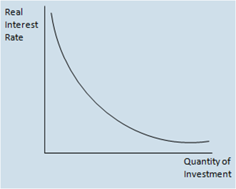Some firms may choose to borrow money to fund their investments, therefore the interest rate is of direct significance, the higher it is the less investment that will occur and vice versa. This means there is an inverse relationship between interest rates and investments, we can see this relationship on the graph to the left. Ergo, we can say, algebraically, that the investment function is:

I = I(r) meaning that investment is a function of investment related to the interest rate.

Interest rates also have an indirect effect. If businesses don’t borrow to invest then they would have to use retained earnings. If the interest rate is high then the firm would be able to save its retained earnings and earn a high level of interest (there is a high opportunity cost of investing rather than saving). Therefore high interest rates again lead to less investment as the return on investment will have to be higher than the interest rate.

When talking about interest rates in the context of investment we are talking about the real interest rate. Normally, in conversation and when reading from figures, the interest rate refers to the nominal rate, however this doesn't include inflation. The real interest rate is the nominal interest rate minus the inflation rate. We use the real interest rate when talking about investment because inflation will eat away at the returns of any investment projects, and hence they need to be included. See interest rates for more information on this.

Taxation affects investment directly as well, as the higher it is, the less retained earnings a firm will have to invest. Indirectly it will reduce the return on investment and thus make investing less attractive. Business confidence is also vital for investment; if it is high there will be more investment and vice versa.

Government Spending

Fiscal policy is the spending, taxation and borrowing undertaken by the government.

The government control on taxation affects AD; by increasing taxation consumer spending and investment is likely to fall as consumers have less disposable income and firms have less retained earnings. Conversely if tax rates fall consumer spending and investment is likely to rise as consumers have more disposable income and firms have more retained earnings. Government spending affects AD by increasing it if government spending rises or remains high and vice versa. Also if the government is spending a lot then people may become more optimistic about the future and so increase spending.

The fiscal stance of the government can either be expansionary where the aim is to increase the output of an economy or contractionary. Generally contractionary fiscal policies occur during an economic boom during fast and unsustainable growth.

There are 2 forms of government spending; automatic and discretionary. Automatic goes against the business cycle for example unemployment benefits and corporation tax. Unemployment benefits keep consumption up even during an economic trough. Corporate tax reduces consumption at high rates therefore reducing the economic peak. These are known as automatic stabilisers.

Discretionary government spending is where the government chooses to spend money for example by aiding first-time home buyers. Government spending is an autonomous component of aggregate demand as certain spending e.g. national security, will occur regardless of income accrued from taxes. 

See Ricardian Equivalence and read more about Government Spending and its affect under Demand Side Policies.

Welfare Payments

When talking about government spending, we don't include the value of welfare payments (benefits) made to people on lower incomes. This is because this is a reallocation of existing income from the rich to the poor, through taxation and welfare payments. Such welfare payments would show up, instead, in the consumption component as people are likely to spend a certain proportion of their income by consuming anyway. Therefore this removes the issue of double counting this money in consumption and government spending.

It is noteworthy that those on benefits generally have a higher marginal propensity to consume than more wealthier people. This is because a larger proportion of their income goes on necessities, or basic luxuries. People on low incomes generally do not earn enough to save, and would rather increase their standard of living by purchasing consumer goods rather than saving money. Hence, this might suggest that increasing welfare payments would result in higher consumption than that which would have occurred if taxation were reduced. This is because people who receive an increase in their welfare payments would be likely to spend more of it (we have just said that they have a relatively high MPC) than richer people who are likely to save more if taxes fall. 

Exports are goods or services that a country sells to another country. Imports are the opposite - goods or services that a country purchases from another country. Imports are seen as bad for an economy, because to purchase an import means money flows out of a country to another economy. However, if the import is a capital good then it can result in an increase in the productive capacity of the domestic economy. Additionally, imports of consumer goods can result in an increase in the standard of living of the population. 

Exports are seen as good for an economy as they result in more money for the population (or at least the owners of capital goods), however if exports deprive the domestic population of consumer goods in order to produce capital goods to produce consumer goods for the export market, then it can cause a lower standard of living. To put it another way, if a country only produces consumer goods to sell to foreigners in order to make income, or only produces capital goods to later produce consumer goods for the export market, then it means that the local population cannot enjoy the products which they have spent so long toiling to make.

From a circular flow point of view, exports are seen as an injection, as they bring money into the economy, whereas imports are seen as a withdrawal, as they result in money flowing out of the economy. Hence the formula for aggregate demand, is exports minus imports. If this component is negative then imports must be greater than exports. Don't forget that imports and exports include more than just goods, services for many economies contribute far more than goods do.

Read more about exports and imports and how they effect the economy here.

Multiplier

The multiplier effect is the process by which any change in a component of AD results in a greater final change in real GDP. When injections exceed leakages, aggregate demand will increase. This increase in AD will have a larger effect on the economy. This is because when people spend money, that expenditure then becomes the income of those who sell them the product, who in turn go out and spend some of the money. Therefore there is a knock on effect which is known as the multiplier. For example £100 of investment will increase AD in the economy by more than £100 (provided MPC isn’t 0) because the initial investment would be spent by those who receive it which would be spent again and then again... and so on!

The lower the number of leakages; the higher the MPC (the lower the MPS) and the less imports into a country, the greater the effect of the multiplier. This means that any change in government spending will have a knock-on effect in the economy providing that the multiplier is greater than 1.

Assume we know the average value of the MPC in an economy, let MPC be 0.6. Let us now say that the government decides to stimulate the economy by injecting an additional £1 million into it by building a new motorway. The £1 million initial injection is spent on materials and wages for the labourers who build the new motorway. But the workers and merchants who have received this income will then go out and spend it. In our situation they will spend 60% of it (as we have said that MPC = 0.6) so they will go and spend £600,000, perhaps by buying their family a gift, or by eating out at restaurants more. These restaurant owners and shop keepers will then go out and spend 60% of the £600,000 they have received (a figure of £360,000) and so on. We can work out the total increase of AD by adding up all these increments: £1,000,000 + £600,000 + £360,000 + £216,000 + £129,600 + £77,760 + £46,656 + £27,993.60 + .... This adds up to a total of £2.5 million. Note: we can work this out by using the formula for the sum of a geometric progression up to infinity which is Sn = a/(1-r). Where a is the initial number (1 million) and r is the ratio (0.6). 

Therefore, in our example the £1 million initial injection into the economy by the government resulted in a total increase of £2.5 million. Hence we can say that the multiplier in this example is 2.5 (final value/initial value). However it is important to note the simplicities in the model we have just demonstrated; firstly, we have used a high MPC, secondly we have assumed that the MPC is constant - we have taken an average MPC, which obviously wouldn't be the case in reality. Within an employment group (e.g. road builders) MPC is likely to differ because people are different and between groups (e.g. a road builder and a shop keeper) MPC will differ due to different standards of living. We also didn't include the number of withdrawals from the circular flow in our model. As well as saving (which was included), taxation and imports are other withdrawals which weren't included in our model. The UK economy imports a lot of goods and so this may greatly reduce the ultimate multiplier value.

A multiplier greater than 1 would, as we have seen, increase GDP assuming an injection of cash. However if the government decides to withdraw cash from the circular flow (by increasing taxes, reducing spending or a mixture of both) then a multiplier greater than 1 would lead to a higher proportional fall in GDP which would be considered a negative multiplier. Therefore in times of austerity GDP would only increase if the multiplier is less than 1, this may because a country imports a lot of goods and hence cutting spending only results in a fall in imports, which although it would hurt other countries' economies, it wouldn't cause as many problems to the domestic economy.

The formula for the multiplier is: 1 / 1 - MPC  

This can be proved using the formula for aggregate demand in a closed economy. AD = C + I + G. This must be national income, as Y = AD; what a country earns must be the same as what is effectively demanded. 

Hence we can say Y = C + I + G; if we substitute in the consumption function: C = a + bY: 

Y = a+bY + I + G;

Dont forget that b is the MPC and a is autonomous consumption. Now let us re-arrange the equation to get:

Y - bY = a + I + G

Factorise:

Y(1 - b) = a + I + G

Divide both sides by (1-b)

Y = a/(1-b) + I/(1-b) + G/(1-b)

This can be written as:

Y = a(1-b) + [1/(1-b)]I + [1/(1-b)]G

Now finally, let us analyse this last equation. If I or G increase then we can see that Y will increase by the same amount. Hence ΔY = 1/(1-b). This is the equation for the multiplier.

We can therefore say that the formula for the change in GDP resulting from an increase in either G or I is equal to the the change in AD (the initial increase as a result of the rise in G or I) multiplied by the formula for the multiplier:

So far we have only spoken about the multiplier resulting from spending. However, there is also a multiplier associated with taxation.

With the spending multiplier, as well as the after effect of the change in spending there is also an initial increase/decrease. If the government adds £1 million to the economy, as well as their being greater income occurring from the multiplier effect, there is also a £1 million boost to the economy. This won't happen with the taxation multiplier, because some portion will be saved.

Say, the government reduces taxes so that every household saves £100 leading to a total tax reduction of £500 million. However, the economy won't grow by £500 million, because this tax saving may be saved by some people, let us say that the Marginal Propensity to Withdraw (MPW - this includes, savings, imports and tax) is 0.4, this means that the MPC is 0.6, hence £200 million will be saved and only £300 million will be spent. Only then, will the multiplier come in to play. Keynes came up with a simple formula to work out the tax cut multiplier: -MPC/MPS. If the government reduce tax (-) then a negative multiplied by a negative is a positive and so the tax cut would increase aggregate demand. If the government increased tax (+) it would result in a negative so aggregate demand would fall.

We can compare the benefits to the economy of a spending increase compared to a tax reduction. Let us assume that MPC is 0.8 (MPW is ergo 0.2), and the government decides to either reduce taxes by £1 billion or increase government spending by £1 billion. Looking at the spending side first the multiplied effect of the £1 billion increase is: [£1bn*1/(1-MPC)]; [1bn*1/(1-0.8)]; [1bn*5] = £5 billion. Now, looking at the tax reduction side, we have £1 billion multiplied by MPC/MPS = £1bn*(0.8/0.2) = £1bn*0.4 = £400 million.

So we can see that in either case the government loses revenue of £1 billion, but if it spent the money it would increase the economy by £5 billion whereas if it gave the money to taxpayers (by reducing taxes) it would only benefit the economy by £400 million. This is a vast difference and this simple model demonstrates that government spending is more effective than tax reduction. According to Keynes, increased government spending always "outperforms" decreases in tax to stimulate the economy.

The government could maintain a balanced budget whilst trying to improve the economy - perhaps during a slump - by increasing spending whilst increasing taxes to pay for the spending increases, hence maintaining a balanced budget. Let us assume that MPC is 0.7 (meaning MPW is 0.3) and the government decides to boost the economy with a £2 billion fiscal injection. It could afford this by depleting a surplus (if it has one), increasing taxes or borrowing. As we have said, in this example the government wants to balance its books, so rather than borrow the money (perhaps interest rates are stifflingly high) it decides to increases taxes by £2 billion to finance the fiscal spree.

The multiplier for the fiscal injection will be (1/0.3)*2bn = £6.66 billion (roughly). This means that by increasing spending by £2 billion the government actually increases GDP by £6.66 billion (an increase of £4bn as a result of the multiplier)!

Now we need to calculate the negative multiplier for the tax increase: -MPC/MPS * tax change = -0.7/0.3*(2bn) = -£4.66bn. Therefore the tax increase means that GDP will fall by £4.66bn.

Finally, we need to calculate the net effect of the tax increase with the spending increase. The economy was injected with a multiplied total of £6.66bn but a multiplied tax withdrawal of £4.66bn was removed from the economy. By subtracting £4.66bn from £6.66bn, we get a net increase of £2bn. This means that the government has a balanced book (it didn't increase its debt, or reduce its surplus) but managed to boost the economy by £2bn simply by using the power of the multiplier, and the fact that the spending multiplier is more powerful than the tax multiplier!

This can work in reverse too though, if the government cut public spending by £x and passed this on to the public by also cutting taxation by £x, then the economy would still contract, due to the differing multiplier effects, even though the value of the withdrawal (cut in public spending) is the same value as that of the injection (cut in taxation).

The balanced budget multiplier is 1; if the government increased spending by £x and increased taxes by £x to balance its budget (and vice versa) then the overall net benefit (or loss) to the economy will be £x.

We can also note that the difference between the value of the government spending multiplier and the taxation (just the value not the effect of the multiplier on the economy) is exactly 1.

Graphs

We have already seen that the aggregate demand curve is downward sloping and explained why. We now focus on shifts in aggregate demand and how they would appear graphically.

Aggregate demand would shift rightwards as a result of an increase in a component of the aggregate demand formula. We can see the effect below. Such an increase in a component could occur for many reasons such as - a fall in interest rates leading to more investment and consumption, a fall in the exchange rate making exports more competitive abroad, an increase in the quality of domestically produced goods resulting in an increase in exports and fewer imports.

It is difficult to analyse the effects of this without seeing the curve for aggregate supply (we will do a complete analysis later on), but we can see that at any point there will be an increase in the price level (inflation - more demand causes prices to rise) and an increase in output/income and the unemployment level.

A leftward shift would occur if a component in aggregate demand were to fall, for example the government might reduce its spending in order to reduce its budget deficit and the public sector net debt. It may also increase taxes to help in this effort which would reduce disposable incomes and potentially the value of consumption. We can see a leftward shift below.

Aggregate Supply

The total quantity of output supplied in an economy over a period of time depends on the quantities of input of factors of production. The ability of firms to vary output in the short run will be influenced by the degree of flexibility the firms have in varying inputs. Therefore it is necessary to distinguish between short-run and long-run aggregate supply.

Short Run

In the short run, firms have very little ability to increase output as a result of increased demand signaled by higher prices. They may find it difficult to hire and train new workers in such short notice in order to increase production to meet the rise in demand. Similarly, they may also find it hard to finance and set up more capital to ramp up production. To combat this they may offer workers more overtime to produce more; this will result in higher costs for the firm which they reflect in higher prices of goods - causing higher price levels. This explains why the short run aggregate supply curve is downward sloping as we can see.

Long Run

However, in the long run firms won't want to be offering too much overtime (as this is expensive) and they will also have had time to have found and trained new workers. Keynesian's believe that the long run aggregate supply curve (LRAS) is upward sloping with 3 distinguished features, as we can see to the left.  

At low levels of real output (towards the left) firms have spare capacity (unused factory space, equipment and workers that are working unproductively) and can increase output easily without paying overtime.

At the point where the curve is no longer elastic (the gradient increases) businesses are trying to increase output using overtime and bonus payments, this increases the cost of production slightly which is why the price level increases. 

At the point where the curve is inelastic/vertical no more output can be obtained without a shift of the LRAS curve. All available resources are fully employed. This is known as the maximum potential output and is the same point as full employment (although not including frictional unemployment). Therefore if the economy where at this point it wouldn't be desirable to have further aggregate demand as this would only cause inflation and wouldn't lead to any increase in output or employment levels.

Monetarists on the other hand, believe that the LRAS curve is perfectly inelastic and that this will shift to reflect improvements in aggregate supply.

Graphs

To increase the level of aggregate supply a factor of production needs to either increase in quantity or improve in quality. For example, an increase in the labour force resulting from immigration would cause a rightward shift of aggregate supply as we can see on the left. This causes more goods to be produced at a lower price level; meaning the population can enjoy more goods at a cheaper price. Conversely a fall in aggregate supply could occur due to outward migration leading to a smaller labour force at home, this is shown on the diagram to the right, resulting in less being produced but at a higher price.

For more on what determines the level of aggregate supply, please read our page on Supply-Side Factors.

Equilibrium

Macroeconomic equilibrium is the price level and amount of real output where the plans of firms to produce and the plans of all elements of aggregate demand coincide. It is the total planned output of an economy, identified by the intersect of AS and AD.

Note that Keynes pointed out that equilibrium isn’t always full employment equilibrium and so may not be beneficial to be at.

We can use an equilibrium model to analyse what would happen if aggregate demand, aggregate supply or both changed to see the effect on the output produced and the price level. 

If aggregate demand were to increase (shift right) we can see (LEFT) that this will cause a rise in inflation but also in output. But if the economy is already at full employment then any further increases in AD will only cause inflation. If the economy is on the elastic section of the LRAS curve then output may increase without the effects of inflation. If aggregate demand were to fall (a leftward shift) we can see (RIGHT) that price levels drop (note: this doesn't necessarily mean a fall in inflation - deflation - but may just mean that the rate of inflation has slowed) but so do the level out output. Thus the negative production gap increases causing more unemployment.

A fall in aggregate supply (a leftward shift) would lead to a rise in price levels and a fall in output produced as we can see on the diagram to the left. The diagram to the right shows us what would happen if aggregate supply were to increase (shift rightwards); we would see a fall in the price levels and a rise in output, both are considered highly desirable.

There are also further variations of outcomes which can be analysed, if both aggregate demand and aggregate supply rise/fall at the same time and by different degrees.

Negative Production Gap

We have just seen that the full employment level is when the economy is operating at the maximum potential output point on the long run aggregate supply curve (the inelastic section). At this point the only unemployment will be frictional as a result of people being out of work to look for other jobs. 

If the economy were operating at another point of the LRAS curve, say point A, then the amount of output produced would be Y₁, therefore there would be a negative production gap of Y₁-Y_F, which can be seen as unemployment. Hence any increase in aggregate demand that would increase overall output nearer to the full employment point would result in a fall in unemployment.

Page last updated on 03/08/15